
Profiling a program consists in dynamically collecting measures during the program execution : which functions or pieces of code are executed, how many times, the duration of an execution, the call tree, …
cProfile is a common profiler for Python programs.
cProfile does deterministic profiling - it collects counters for the whole program execution - as opposed to statistical profiling that monitors samples of the program execution. py-spy (statistical), yappi (deterministic), etc. are other options for Python profiling.
Other options for profiling include system level profiling tools (eg with perf for Linux), or advanced commercial multi-langage profilers such as Alinea map and Intel Vtune for which Inria has licences.
cProfile lets you easily profile your whole script and save result to an output file (cprofile.out here) in pstats format with :
[user@laptop $] python -m cProfile -o cprofile.out /path/to/my_script.py
For profiling a section of your Python script, simply instrument the code with :
import cProfile profile = cProfile.Profile() # start profiling section profile.enable() # place your payload here my_profiled_code_or_function() # stop profiling section profile.disable() # save collected statistics profile.dump_stats('cprofile.out')
You can then install a profiling data viewer such as snakeviz and run it on the profiling data :
[user@laptop $] snakeviz cprofile.out
A more basic option is to use the pstats module interactive mode :
[user@laptop $] python -m pstats cprofile.out Welcome to the profile statistics browser. cprofile.out% stats 5
You may also use the profiling data programatically by further instrumenting your script eg :
import pstats profile_stats = pstats.Stats(profile) # print to stdout top 10 functions sorted by total execution time profile_stats.sort_stats('tottime').print_stats(10) # print to stdout top 5 functions sorted by number of time called profile_stats.sort_stats('ncalls').print_stats(5)
Here is an example of a snakeviz view for a geomstats hypersphere metric norm computation :
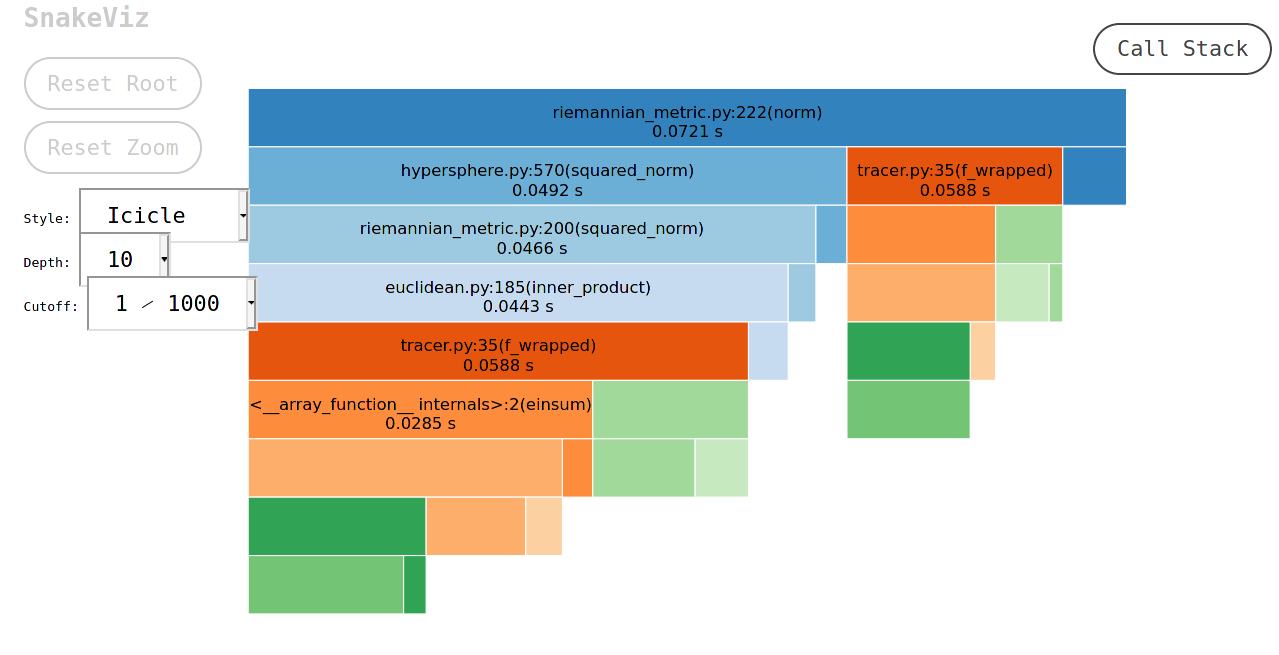
… and text output for top 5 functions sorted by total execution time, for the same computation :
Ordered by: internal time List reduced from 16 to 5 due to restriction <5

ncalls tottime percall cumtime percall filename:lineno(function)
20000 0.017 0.000 0.059 0.000 /user/mvesin/home/.conda/envs/geomstats-conda3backends/lib/python3.7/site-packages/autograd/tracer.py:35(f_wrapped) 10000 0.013 0.000 0.013 0.000 {built-in method numpy.core._multiarray_umath.c_einsum} 20000 0.008 0.000 0.013 0.000 /user/mvesin/home/.conda/envs/geomstats-conda3backends/lib/python3.7/site-packages/autograd/tracer.py:65(find_top_boxed_args) 10000 0.008 0.000 0.026 0.000 {built-in method numpy.core._multiarray_umath.implement_array_function} 10000 0.005 0.000 0.072 0.000 /home/mvesin/GIT/geomstats/mvesin_geomstats/geomstats/geometry/riemannian_metric.py:222(norm)

210006 function calls in 0.072 seconds
When analyzing profiling results, you often want to focus on functions with higher cumulative time (time spent in function and its sub-functions - those at the top of the call hierarchy) or total time (time spent only in function - those where the heavy work takes place). Look also at the number of calls of a function (is it long to execute or often called ? does it match what is expected or does it suggest un-needed calls ?) and to the function call hierarchy (who calls who ?).
You may also want to replay execution step by step with a Python debugger such as pdb to help link profiling results with the execution flow.
cProfile profiling was recently used by EPIONE team and SED-SAM recently for jointly tuning geomstats performanc. It helped better understanding performance trends and gaining significant acceleration for parts of the library.